How to Unhide Columns in Excel

When you have some data columns that you don’t want to display can be hidden from the sheet. The hidden columns can be identified because the numbers are skipped and a double line will be displayed when the cursor is on the place of the hidden columns.
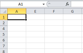
When it comes to unhide the columns, there are a few ways to do it as explained below.
Unhide first column
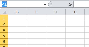
1. Type ‘A1’ in the ‘Name Box’ and press Enter Key to select the first hidden column.
2. Then go to ‘Home’ tab > ‘Format’ button to get the dropdown menu.
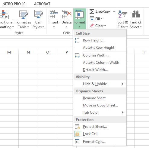
3. Then go to ‘Visibility’ > ‘Hide & Unhide’ > ‘Unhide Column’
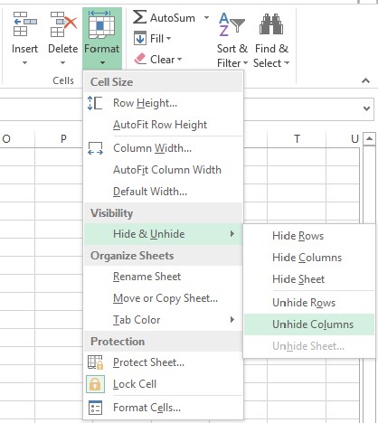
4. Now, the first column is unhidden. This method can also be used to unhide any single column.
Unhide other single or multiple column/s
1. Identify the hidden column/s and select the from a left column to right beyond the hidden column/s. Not necessary to select the immediate left or right columns. In the example we have selected column E to I.
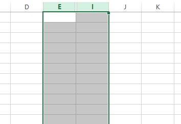
2.Then right click on the title cells of the selected columns to get the list of options.
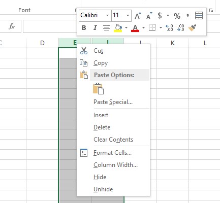
3. Go to ‘Unhide’ option and click it to unhide the hidden columns.

Unhide all columns
1. There may be hidden columns in different places.
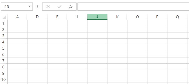
2. Select all columns by clicking top left arrow as shown below.
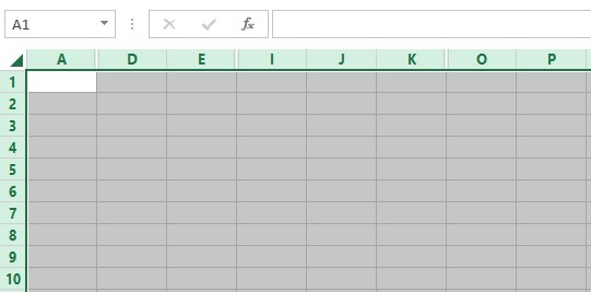
3. Then right click on one of the columns and follow the instructions as explained previously.
Additional useful information
-
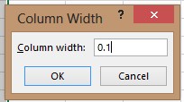
Some columns may not still appear if the column width has been set to a very small value (eg. 0.1). Then you won’t see it as a normal column.
-
-
Select from left to right (or right to left) columns including the one not visible. Then give a common value for ‘Column Width’ which is larger enough to see.
-
Also to widen the columns place the cursor on the right corner of the column and drag to increase the column width.


