The Sparkline in Excel is a tiny chart, which can be included within the background a cell. This is used to provide visual representation of data, showing the variations, minimum/ maximum values and data trends.

A few sample Sparklines are shown below.

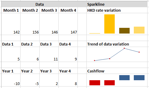
The use of Sparkline is useful because it can show graphical representation of data trends and patterns, next to the data cells. However, it is not necessary to place the Sparkline next to the data cells.

How to add a Sparkline

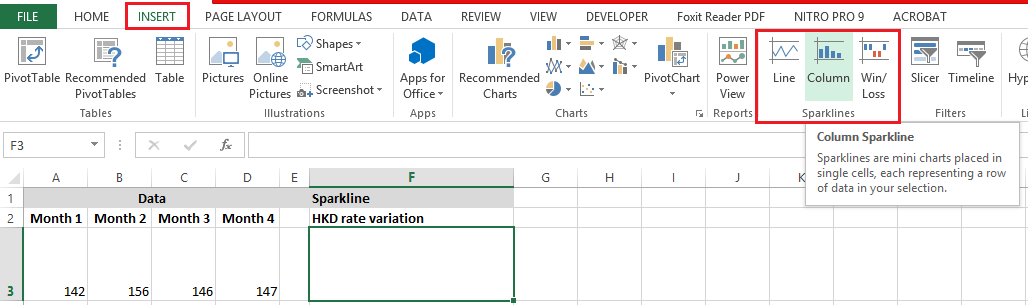
1. Select a cell where you want insert a Sparkline, Go to Insert > Sparklines > Select one of the Sparkline type you want, depending on the required data interpretation (Line, Column, Win/Loss)

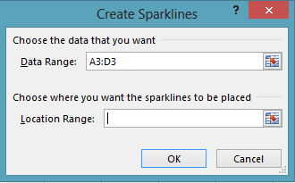
Then choose the data cells that you want to add to the Sparkline.

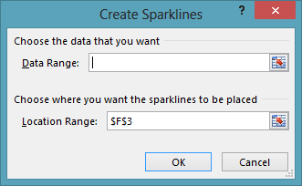
Click OK

1. Or you can first select the data cells and then go to Sparklines > now you have to enter the location (i.e. cell) where the Sparkline to be placed.

2.  

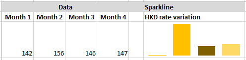
Once you insert the Spakline, you can do changes such as add color schemes, styles, markers etc. This can be done under Design tab. The Design tab will become available when the Sparkline is selected.

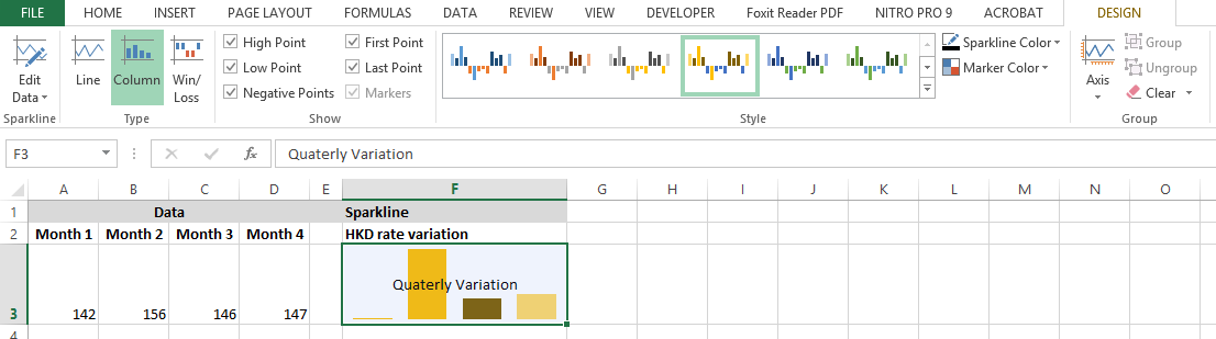
As mentioned earlier, the Sparkline is placed in the background of the cell. Therefore, you still can type anything in the cell.

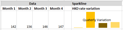
You also can change the dimensions (height of the row and length of the column) of the cell that contains the Sparkline to make the Sparkline clear enough or adjust to the size you want.

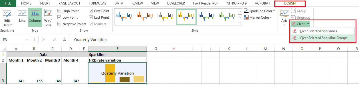
Clear/ Delete a Sparkline 

Select the cell or cells that contain Sparklines > go to Design tab > Click on Clear button