SUMPRODUCT is yet another function that comes to rescue, whether we want to validate a criteria or want to sum against a list of requirements. This function belongs to the SUM family of functions, but differs from usual SUMIFs in that it is an array function.

The uses of SUMPRODUCT are numerous and the use is only restricted by the ingenuity of the user. Most of the time, when you are stuck with validating and data and then summing up something agiant it, you will be referring to this function.

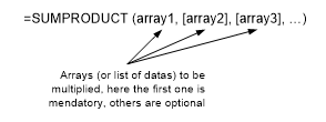
The Syntax:

The function takes at least one argument – an array (range of data) and can take up to 255 arguments in the Que. The arrays must be of same length i.e. number of members in each must be the same. The function works by multiplying the respective members and then summing up the results to give the final result. If there is only array, the formula will simply work as SUM() or more precisely, will multiply the array with an array of 1s to give the answer.

The Simplest Example:

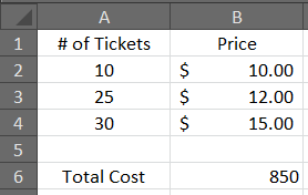
This is perhaps the simplest use of SUMPRODUCT () where you want a weighted total of two quantities. In the following example, the no. of tickets needed to be multiplied by respective prices and the result needed to be summed.

If done manually, it would have taken a whole helper column and the SUM() formula to sum the values, the SUMPRODUCT() formula will do it at once.

=SUMPRODUCT(A2:A4,B2:B4).

Validating Criteria with SUMPRODUCT():

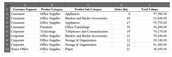
Let’s consider another example to see how SUMPRODUCT() for validating criteria. Referring to the data in the Sheet2, we can find the total sales for a specific Customer Segment and Product Category. For example we want to find the total sales for Corporate Segment and for Office Supplies.

The formula that works for the above data is:

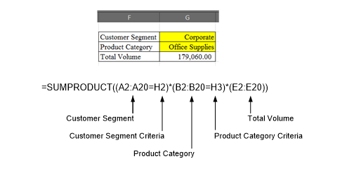
=SUMPRODUCT((A2:A20=G2)*(B2:B20=G3)*(D2:D20))

The formula works by validating if Customer Segment is Corporate; this is done by checking range A2:A20 against criteria in G2. The second validation is done by checking for Product Category in range B2:B20 againt our requirement in cell G3. This entire process returns an array of zeros and ones, and this array is multiplied with values in Total Volume and the result is summed to give the final answer.

Using SUMPRODUCT () to validate for “greater then” and “less than” criteria:

Assuming that you want to find how many times the order quantity crossed the significance level of 10 and lays between maximum of 25 and summing up the corresponding Total Volume. You can also use the SUMPRODUCT () function to get the answer. The formula used for this case is =SUMPRODUCT((D2:D20>=H6)*(D2:D20<=H7)*(E2:E20)).

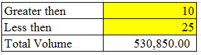
The formula works by checking the range D2:D20 for values greater then threshold value in H6 and repeating the same process if values are less then maximum value in cell H7 and returning an array of ones and zeros and then multiplying it with corresponding sales volume. The result is then summed up to give the final answer.