Using Measures Power Pivot

Measures is a very powerful and vital feature in Power Pivot.
Measures are fields that have been calculated in the 2013 version of Microsoft Excel and have been included in a Pivot Table.
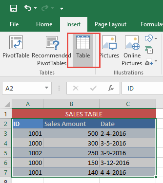
Here is an easy examples on how your first measure can be added to your Pivot bable
Highlight Sales Table, click on the Insert tab, then table and select OK
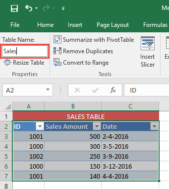
After that, you click on Table Tools, select design and then table name. Give a name that is descriptive to the table. In this instance, sales will be the name we will assign to the table.
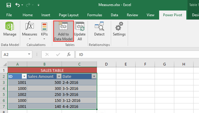
For the 2013 and 2016 versions of Microsoft Excel
Highlight the sales table, click on the Power Pivot tab and select Add to Data Model
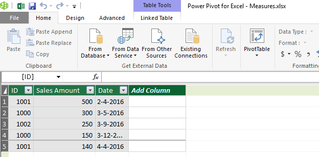
Your table, which in our case was named sales, will be imported into the Window for Power Pivot
For the 2010 version of Microsoft Excel
Click on the Power Pivot Tab and select Create Linked Table
This will result in the window for Power Pivot being opened.
The table named sales will then be loaded to the Data Model for Power Pivot automatically.
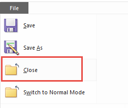
You can now close Window for Power Pivot.
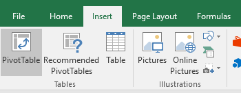
Go to the Insert tab and select Pivot Table
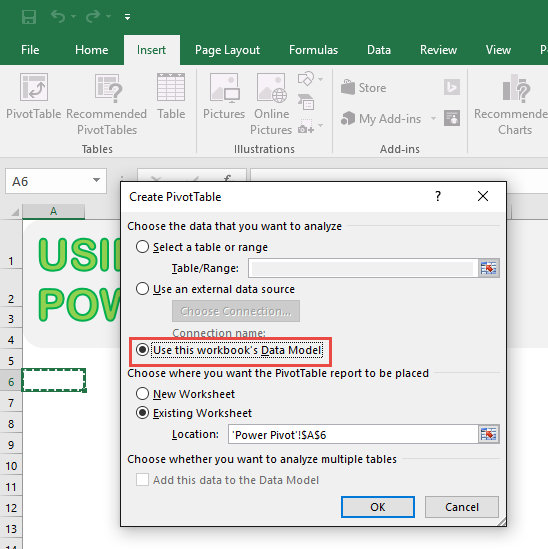
For the 2016 version of Microsoft Excel
Pick the option labeled as Use this workbook’s data model. The data model that was uploaded previously will be used.
Choose the option labeled existing worksheet and select where you want the Pivot Table to be placed, and then select OK.
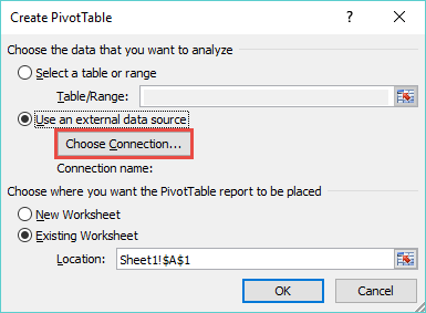
For the 2013 version of Microsoft Excel
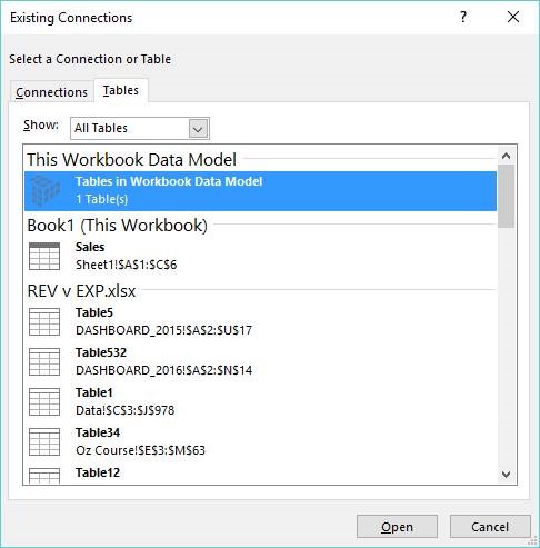
Click on the option labeled Use External Data Source and then select Choose Connection

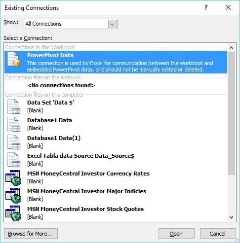
Next, you click on Tables, choose This Workbooks Data Model and then select Open
For the 2010 version of Microsoft Excel
Click on the option labeled Use External Data Source and then select Choose Connection
Now click on Power Pivot Data and select Open
Measure addition
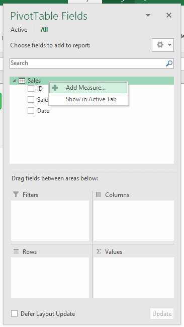
In the 2016 version of Microsoft Excel
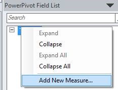
Right click on the Sales Table and select Add Measure
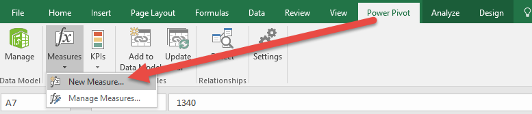
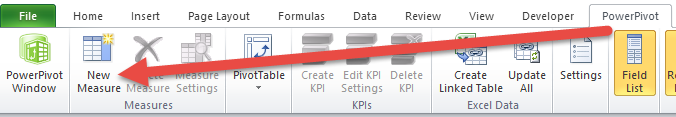
Alternatively, from the Power Pivot tab, click on measures and then click on New measures
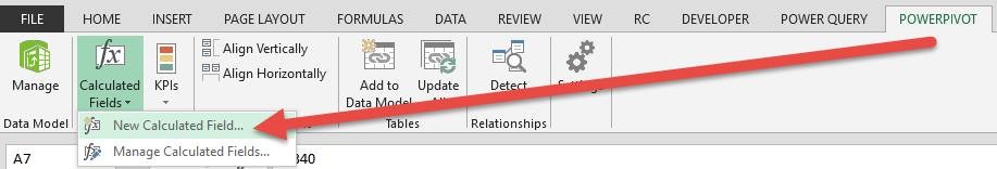
For the 2013 version of Microsoft Excel, choose the Power Pivot tab, click on Calculated Fields and then select new calculated Field.
In the 2010 version of Microsoft Excel
Click on Add New Measure after right clicking the sales table
Alternatively, click on a cell in the Pivot Table, go to the Power Pivot tab and select New measure
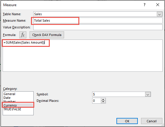
Our 1st measure is created here
You can give Total Sales or any other name as the name for the measure
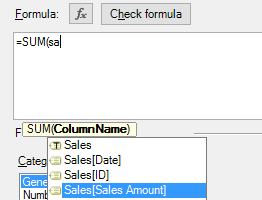
Type =SUM as the formula and select the sum option from the options
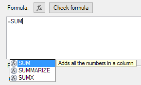
This will give you the helper for formula where you can choose Sales[Sales Amount] and then close bracket.
Use currency for the category and select OK
Put the created Measure in the area for Values
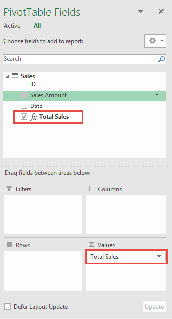
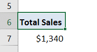
The created Measure can now be used in the Pivot Table

Related Tutorials

Measures is amongst the most important and highly powerful features in Power Pivot. Measures are actually the calculations or formulas you add to the ...

Power Pivot is basically an Excel tool that was first introduced to the public in the year 2010. What exactly is meant by Pow...


Latest
-
Understanding How HYPERLINK Works In Excel
Excel has a built in function to create hyperlinks &...
-
Understanding how MS Excel Query Works
“Query” in MS Excel has same meaning as ...
-
An Introduction To Excel Power Map
Our today’s post is about “Power Map&rdq...
-
Using Pivot Charts For Displaying Data
Conventional charts are mostly used for displaying r...
-
Using “Calculated Items” For Analyzing A Pivot Table
In our last post, we explored how to use calculated ...